In this blog, we use the Structural Topic Model (STM) to analyze the effect of gender on Ph.D. students’ choice of research topics in economics in France. STM integrates probabilistic topic modeling with regression analysis to examine how document metadata influences two key aspects of the topic model: topic content and topic prevalence. If you are not familiar with probabilistic topic models, we recommend reviewing the first blog post and the related references for background information before proceeding.
In this blog post, we examined how the year of defence influences the prevalence of a topic, i.e. the probability that this topic is used during this year. The underlying intuition is that thesis topics are strongly shaped by the period in which they are written; what is considered a contribution evolves alongside the social and academic context of a given time.
However, this approach can be refined further. When predicting topic prevalence using the year of defence, we acknowledge this “evolving social context” but do not specify the mechanisms driving these changes. Additional variables could provide a clearer explanation of authors’ topic choices. For instance, one of the most significant transformations in the French Ph.D. landscape is the increasing proportion of women pursuing doctoral degrees in economics. Are there research topics that male Ph.D. students are more likely to explore, while female Ph.D. students tend to focus on others?
Let’s explore this issue!
Exploring the data
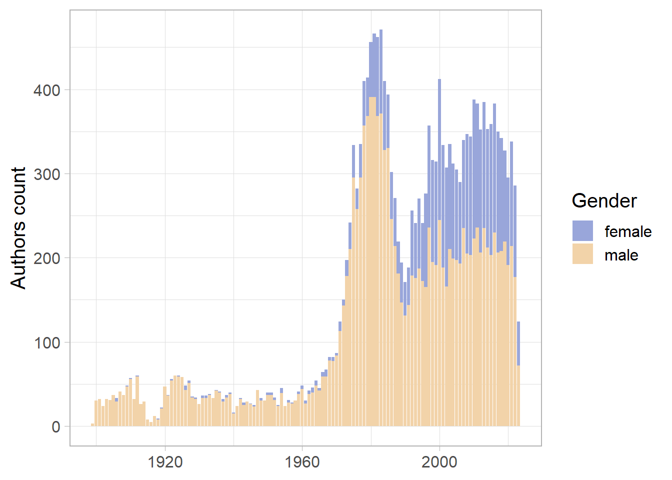
To run our topic model, we use the abstracts (abstract_fr) as the main textual input. As previously explained here, abstracts provide significantly better data than titles for training a topic model; however, they are only available from the early 1980s. Consequently, we limit our analysis to the past four decades. This period also marks a sharp increase in the proportion of female authors, making it particularly relevant for examining gender dynamics in academic publishing.
Let’s explore the data to analyze the gender distribution in the French Ph.D. dataset. The individuals table includes two distinct variables, gender and gender_expanded, which provide information about the gender of individuals (e.g., authors, supervisors).
The gender variable contains raw information obtained from the IdRef database.
The gender_expanded variable is our enhanced version, which imputes missing gender values using French census data.
More information on these variables can be found in the documentation of the French database available on this website. For this analysis, we will use the gender_expanded variable.
The gender_expanded variable is derived from the thesis_individual table, whereas our textual data come from the thesis_metadata table. To link these variables, we must use the thesis_edge table, which associates each thesis identifier (thesis_id) with the corresponding entities (entity_id), and so to the author of the thesis.
Show the code
thesis_metadata <-readRDS(here(FR_cleaned_data_path, "thesis_metadata.rds"))thesis_individual <-readRDS(here(FR_cleaned_data_path, "thesis_individual.rds")) # Show sample of each tables for illustration # set seed set.seed(123)# Sample data from thesis_metadatametadata_sample <- thesis_metadata %>%select(thesis_id, abstract_fr, year_defence) %>%filter(!is.na(abstract_fr)) %>%mutate(abstract_fr =str_trunc(abstract_fr, 10)) %>%slice_sample(n =5)# Sample data from thesis_individualindividual_sample <- thesis_individual %>%select(entity_id, entity_name, entity_firstname, gender_expanded) %>%slice_sample(n =5)# Convert samples to datatablesmetadata_table <-datatable(metadata_sample, options =list(pageLength =5,searching =FALSE,lengthChange =FALSE), caption =" Metadata")individual_table <-datatable(individual_sample, options =list(pageLength =5,searching =FALSE,lengthChange =FALSE), caption =" Individuals")# Display tables side by side using HTMLhtmltools::browsable( htmltools::tagList( htmltools::tags$div(style ="display: flex; gap: 20px;", htmltools::tags$div(style ="flex: 1;", metadata_table), htmltools::tags$div(style ="flex: 1;", individual_table) ) ))# Join them with edge tablethesis_edge <-readRDS(here(FR_cleaned_data_path, "thesis_edge.rds"))authors_doc_id <- thesis_edge %>%filter(entity_role =="author") %>%select(entity_id, thesis_id) %>% uniqueauthors_gender <- thesis_individual %>%select(entity_id, entity_name, entity_firstname, gender_expanded)# manage duplicateduplicates <- thesis_metadata %>%filter(!is.na(duplicates)) %>%group_by(duplicates) %>%# when the line has a duplicate, group and keep the older valueslice_max(year_defence, n =1, with_ties =FALSE)thesis_metadata_no_duplicate <- thesis_metadata %>%filter(is.na(duplicates)) %>%bind_rows(duplicates)# We can now select the relevant variables for our stmdata <- thesis_metadata_no_duplicate %>%# keep relevant columnsselect(thesis_id, abstract_fr, year_defence) %>%# double join to add a gender to each documentleft_join(authors_doc_id, by ="thesis_id") %>%left_join(authors_gender, by ="entity_id")
Table 1: Sample of metadata and individual tables
We can now evaluate the distribution of our data. Figure 1 illustrates the distribution of theses, categorized by gender.
data <- data %>%filter(!is.na(gender_expanded), !is.na(year_defence))gg <- data %>%group_by(gender_expanded, year_defence) %>%summarise(n =n()) %>% ungroup %>%mutate(tooltip =paste("Année:", year_defence, "<br>Nombre d'auteurs:", n, "<br>Genre:", gender_expanded)) %>%ggplot(aes(x =as.integer(year_defence),y = n,fill = gender_expanded,text = tooltip )) +geom_col() +theme_light() +labs(x =NULL, y ="Authors count", fill ="Gender") +scale_fill_scico_d(begin =0.3, end =0.9, palette ="oleron") +theme_light(base_size =15)print(gg)
Figure 1: Distribution of PhD by gender
Show the code
distribution <- data %>%group_by(gender_expanded, year_defence) %>%summarise(n =n()) %>% ungroup distribution %>% DT::datatable(extensions ='Buttons',options =list(dom ='Blfrtip',buttons =c('excel', 'csv'),pageLength =10 ),filter ='top'# Adds a search bar for each column at the top )
Table 2
Gender of theses’ authors per year
The practice of including an abstract became common in the early 1980s, but few abstracts were available for theses defended in earlier decades. A closer examination shows, however, that these were added by librarians who created the entries. Therefore, it is reasonable to filter out theses defended before 1980.
To run our probabilistic topic model, we follow the usual pre-processing steps, as described in this post. The primary difference in this instance is the removal of a few custom stopwords to address highly redundant terms frequently found in abstracts, such as “chapitre” (chapter) or “thèse” (thesis). We can then run the topic model. For a corpus of 11,000 abstracts, starting with \(K=100\) (the number of topics) provides a reasonable basis for exploration.
Show the code
# ----------------------------------# STEP 1: DATA PREPARATION# ----------------------------------# Retain only rows with a gender # Retain only rows with an abstract# Retain only rows after 1980data <- data %>%filter(!is.na(gender_expanded),!is.na(abstract_fr), year_defence >1979 )# ----------------------------------# STEP 2: TOKENIZATION AND PARSING# ----------------------------------# Initialize the spaCy model for French# Ensure spaCy is installed and the French language model is downloaded.# spacy_install(force = TRUE)# spacy_download_langmodel("fr_core_news_lg", force = TRUE)spacy_initialize("fr_core_news_lg") # Parse titles using spaCy# Perform pre-cleaning on French abstractsparsed <- data %>%# some pre-cleaning of abstractmutate(abstract_fr =str_to_lower(abstract_fr),abstract_fr =str_replace_all(abstract_fr, "", " ") %>%str_replace_all(., "", " "),abstract_fr =str_remove_all(abstract_fr, "$\\(?Résumé"),abstract_fr =str_replace_all(abstract_fr, "-", " "),abstract_fr =str_squish(abstract_fr)) %>%pull(abstract_fr) %>%# identify words spacyr::spacy_parse(multithread =TRUE)# Map thesis IDs to the parsed tokensid <- data %>%distinct(thesis_id) %>% ungroup %>%mutate(doc_id =paste0("text", 1:n()))parsed <- parsed %>%left_join(id, join_by(doc_id)) %>%select(-doc_id)saveRDS(parsed, here(website_data_path, "parsed.rds"), compress =TRUE)# ----------------------------------# STEP 3: TOKEN FILTERING AND CLEANING# ----------------------------------parsed <-readRDS(here(website_data_path, "parsed.rds"))# prepare stop_wordsstop_words <-bind_rows(get_stopwords(language ="fr", source ="stopwords-iso"),get_stopwords(language ="fr", source ="snowball"),# some titles have english expressionget_stopwords(language ="en", source ="snowball")) %>%distinct(word) %>%pull(word)# add custom stopwords custom_stop_words <-c("chapitre", "thèse","montrons","montre","analyse")stop_words <-c(stop_words, custom_stop_words)parsed_filtered <- parsed %>%# Count original idsmutate(original_count =n_distinct(thesis_id)) %>%# Filter empty tokens and track removed idsfilter(!pos %in%c("PUNCT", "SYM", "SPACE")) %>%mutate(after_filter1 =n_distinct(thesis_id)) %>% { message("Doc removed after filter: ", unique(.$original_count) -unique(.$after_filter1)); . } %>%# remove special character filter(!token %in%c("-", "δ", "α", "σ", "γ", "東一")) %>%mutate(after_filter2 =n_distinct(thesis_id)) %>% { message("Doc removed after filter: ", unique(.$after_filter2) -unique(.$after_filter1)); . } %>%# remove any digit token (including those with letters after digits such as 12eme)filter(!str_detect(token, "^\\d+.*$")) %>%mutate(after_filter3 =n_distinct(thesis_id)) %>% { message("Doc removed after filter: ", unique(.$after_filter3) -unique(.$after_filter2)); . } %>%# Remove pronouns and french truncmutate(token =str_remove_all(token, "^[ld]'"),token =str_remove_all(token, "[[:punct:]]")) %>%# Filter single letters and stopwordsfilter(str_detect(token, "[[:letter:]]{2}")) %>%mutate(after_filter4 =n_distinct(thesis_id)) %>% { message("Doc removed after filter: ", unique(.$after_filter3) -unique(.$after_filter4)); . } %>%# filter list of stop words filter(!token %in% stop_words) %>%mutate(after_filter5 =n_distinct(thesis_id)) %>% { message("Doc removed after filter: ", unique(.$after_filter5) -unique(.$after_filter4)); . } %>%# Create bigramsgroup_by(thesis_id, sentence_id) %>%mutate(bigram =ifelse(token_id <lead(token_id), str_c(token, lead(token), sep ="_"), NA)) %>%ungroup()# ----------------------------------# STEP 4: BIGRAM CREATION AND FILTERING# ----------------------------------# Create and filter bigrams based on frequency and PMIbigrams <- parsed_filtered %>%select(thesis_id, sentence_id, token_id, bigram) %>%filter(!is.na(bigram)) %>%mutate(window_id =1:n()) %>%add_count(bigram) %>%filter(n >10) %>%separate(bigram, c("word_1", "word_2"), sep ="_") %>%filter(if_all(starts_with("word"), ~! . %in% stop_words))bigram_pmi_values <- bigrams %>%pivot_longer(cols =starts_with("word"), names_to ="rank", values_to ="word") %>%mutate(word =paste0(rank, "_", word)) %>%select(window_id, word, rank) %>% widyr::pairwise_pmi(word, window_id) %>%arrange(item1, pmi) %>%filter(str_detect(item1, "word_1")) %>%mutate(across(starts_with("item"), ~str_remove(., "word_(1|2)_"))) %>%rename(word_1 = item1,word_2 = item2,pmi_bigram = pmi) %>%group_by(word_1) %>%mutate(rank_pmi_bigram =1:n())bigrams_to_keep <- bigrams %>%left_join(bigram_pmi_values) %>%filter(pmi_bigram >3) %>%mutate(bigram =paste0(word_1, "_", word_2)) %>%distinct(bigram) %>%mutate(keep_bigram =TRUE)parsed_final <- parsed_filtered %>%left_join(bigrams_to_keep) %>%mutate(token =if_else(keep_bigram, bigram, token, missing = token),token =if_else(lag(keep_bigram), lag(bigram), token, missing = token),token_id =if_else(lag(keep_bigram), token_id -1, token_id, missing = token_id)) %>%distinct(thesis_id, sentence_id, token_id, token)term_list <- parsed_final %>%rename(term = token)saveRDS(term_list, here(website_data_path, "term_list.rds"))# ----------------------------------# STEP 5: STM INPUT PREPARATION# ----------------------------------term_list <-readRDS(here(website_data_path, "term_list.rds"))# stm object with covariate metadata <- term_list %>%distinct(thesis_id) %>%left_join(data, by ="thesis_id") %>%mutate(year_defence =as.numeric(year_defence)) %>%distinct(thesis_id, abstract_fr, year_defence, gender_expanded) %>%# filter lines with na covariates filter(!is.na(abstract_fr),!is.na(gender_expanded), !is.na(year_defence))# Convert term list to STM-ready formatcorpus_in_dfm <- term_list %>%# remove observations deleted by the metadata filter filter(thesis_id %in% metadata$thesis_id) %>%add_count(term, thesis_id) %>%cast_dfm(thesis_id, term, n)corpus_in_stm <- quanteda::convert(corpus_in_dfm, to ="stm", docvars = metadata)saveRDS(corpus_in_stm, here(website_data_path, "corpus_in_stm.rds"))# ----------------------------------# STEP 6: RUNNING THE STM# ----------------------------------corpus_in_stm <-readRDS(here(website_data_path, "corpus_in_stm.rds"))formula_str <-paste("~", "gender_expanded + s(year_defence)")formula_obj <-as.formula(formula_str)stm <-stm(documents = corpus_in_stm$documents,vocab = corpus_in_stm$vocab,prevalence = formula_obj,data = corpus_in_stm$meta,K =100,init.type ="Spectral",verbose =TRUE,seed =123 )saveRDS(stm, here(website_data_path, "stm.rds"))
Analysis
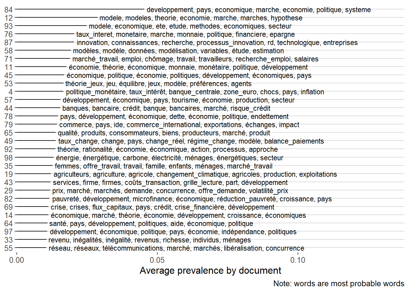
Figure 2 presents the top 20 topics ranked by average prevalence. For each topic, the most probable words from the topic content (based on the \(\beta_{1:K}\) distributions) are assigned. Unsurprisingly, the top topics closely align with common subfields in economics, such as development economics, monetary economics, and the economics of innovation.
Notably, the topics appear more interpretable than those generated by the other model we ran with title_fr. This can be attributed both to the use of a richer source of information and to the fact that we are covering a more recent period, in which topics are more recognizable to contemporary audiences.
Show the code
stm <-readRDS(here(website_data_path, "stm.rds"))label_topic <-labelTopics(stm, n =5) top_terms_prob <- label_topic %>% .[[1]] %>%as_tibble() %>%reframe(topic_label_prob =pmap_chr(., ~paste(c(...), collapse =", "))) %>%mutate(topic =row_number()) # tidy call gamma the prevalence matrix, stm calls it theta theta <- broom::tidy(stm, matrix ="gamma") %>%# broom called stm theta matrix gamma left_join(top_terms_prob, by ="topic") #### plot summary of topics ####theta_mean <- theta %>%group_by(topic, topic_label_prob) %>%# broom called stm theta matrix gamma summarise(theta =mean(gamma)) %>% ungroup %>%mutate(topic =reorder(topic, theta)) %>%slice_max(theta, n =30)theta_mean %>%ggplot() +geom_segment(aes(x =0, xend = theta, y = topic, yend = topic ),color ="black",size =0.5) +geom_text(aes(x = theta, y = topic, label = topic_label_prob),hjust =-.01,size =3 ) +scale_x_continuous(expand =c(0, 0),limits =c(0, max(theta_mean$theta)*3.04), ) + ggthemes::theme_hc() +theme(plot.title =element_text(size =8)) +labs(x ="Average prevalence by document",y =NULL,caption ="Note: words are most probable words" )
Figure 2: Top 30 topics by prevalence
Effect of gender
Now that we have estimated our topics and ensured their interpretability, we can examine the extent to which the author’s gender predicts topic prevalence for a given document. Given the increasing number of female authors over time, topics that are more prevalent in recent theses are more likely to be associated with female authorship. Therefore, we include the year of defense in the regression to distinguish between trendy recent topics and topics more commonly chosen by female authors:
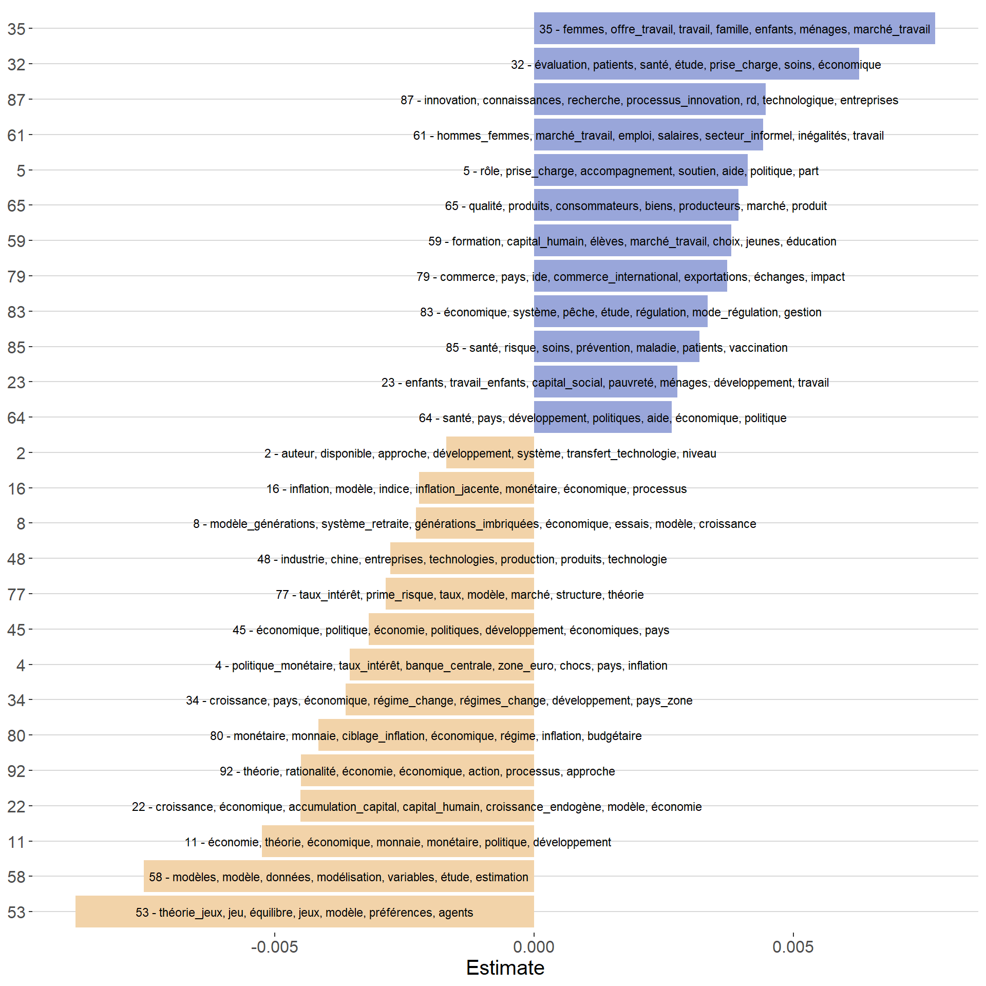
Figure 3 presents the significant estimates for the covariate gender_expanded (with a p-value < 0.1). The y-axis represents the topics, while the x-axis shows the effect of being female on the expected topic prevalence. For instance, being a woman increases the prevalence of topic 35 in a document by 0.0077. Given that the average prevalence of topic 35 is around 0.012, this effect accounts for a significant proportion of the topic’s overall prevalence.
Figure 3: Estimate effect of being a female author on topic prevalence
The first obvious conclusion from this analysis is the presence of a strong gender element in the choice of thesis topics. Male authors are more likely to work on theoretical topics, particularly in macroeconomics, whereas female authors are more associated with applied topics, especially in the fields of health, labor, and education.
Note also that while women tends to work on more applied and empirical issue, the topic 58 about theoretical econometrics is strongly associated to men. This is one of the strength of topic model that is able to differentiate between applied econometric topics and theoretical econometric topics.
Interactions between year and gender
For a more detailed historical analysis, it is also possible to look for an interaction effect between year_defence and gender_expanded in the regression if you are interested in exploring how gender-based topic choices evolve over time:
For instance, certain topics may have been strongly associated with one gender in the early 1980s before becoming neutral or even dominated by the other gender. Here, the estimate gives, for each value of year_defence, the effect of being female on the expected prevalence of a given topic.
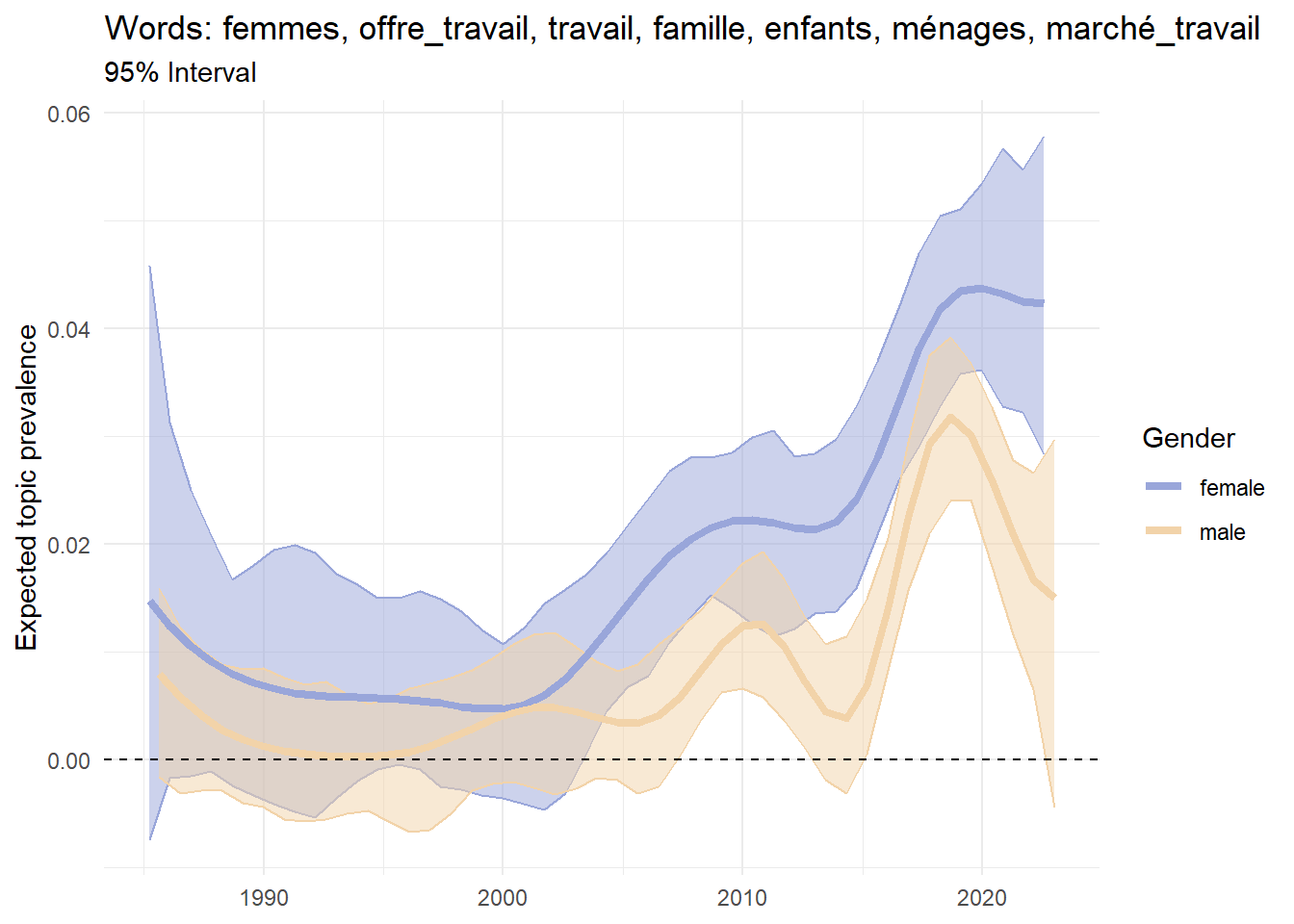
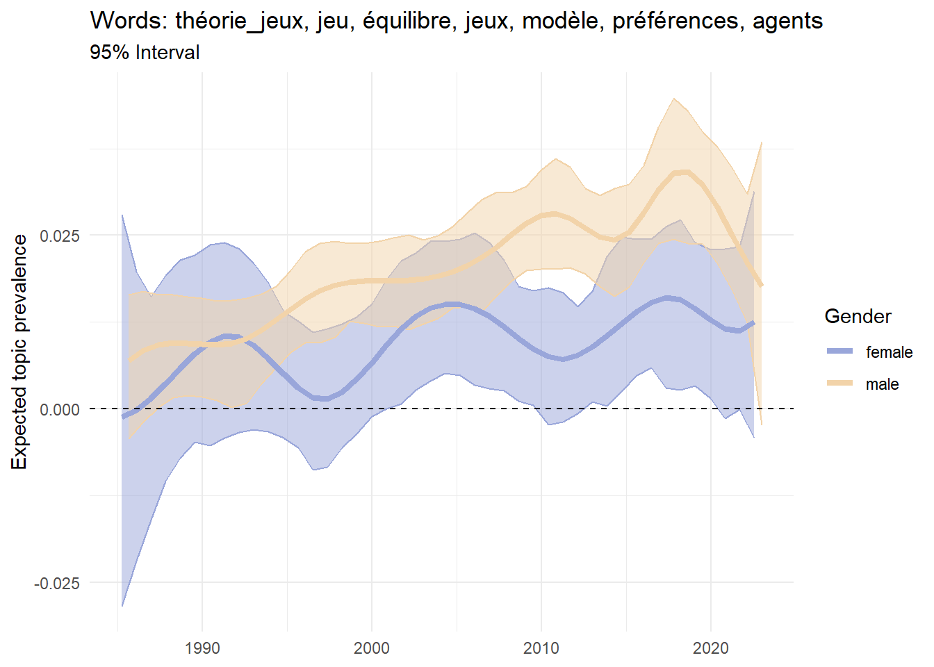
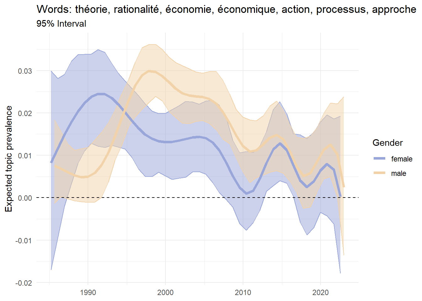
Figure 4 presents the results of such an analysis. For each year_defence and gender_expanded, we compute the expected topic prevalence of topics 35, 53 and 92. Topics 35 and 53 are examples of topic prevalence strongly associated with women and men, respectively. Topic 92 provides a different pattern: while this topic is generally associated with male authors, it was mostly prevalent in women’s theses until the mid-1990s.
Figure 4: Regression of prevalence with interaction
Interactions are particularly interesting for at least two reasons. First, as shown by topics 35 and 53 in Figure 4, gender segregation in the choice of research topics is a very current phenomenon. Second, in the case of Topic 92, interactions allow historical analysis for capturing changes in the gender effect across time. A research area dominated by men today may have been initiated by women in the past, and vice versa.
To conclude, while the regression shows clear gender segregation across fields, it does not answer the question of why this segregation occurs. This phenomenon could be explained by various interdependent factors (Sierminska and Oaxaca 2022; Iaria, Schwarz, and Waldinger 2022). The decision to enter a particular field is “the culmination of a series of earlier decisions” (Strober and Reagan 1976: 304) that depend on students’ socialization, preferences, and the existing opportunities or barriers. Fully addressing this question would require more detailed prosopographical data on Ph.D. students, which is beyond the scope of this blog post.
References
Iaria, Alessandro, Carlo Schwarz, and Fabian Waldinger. 2022. “Gender Gaps in Academia: Global Evidence Over the Twentieth Century.”SSRN Electronic Journal. https://doi.org/10.2139/ssrn.4150221.
Sierminska, Eva, and Ronald L Oaxaca. 2022. “Gender Differences in Economics PhD Field Specializations with Correlated Choices.”Labour Economics 79: 102289.
Strober, Myra H, and Barbara B Reagan. 1976. “Sex Differences in Economists’ Fields of Specialization.”Signs: Journal of Women in Culture and Society 1 (3, Part 2): 303–17.